What Are Images, Really?
Sure, we all know what an image is — it's that cat meme, your phone wallpaper, the thumbnail you forgot to optimize. But under the hood, every image is just a grid of tiny colored squares called pixels. And each of those pixels is defined by three numbers: Red, Green, and Blue (RGB). That's it. Welcome to the matrix.
These pixels are stored in files using different formats — each with its own way of compressing, saving, and occasionally ruining your precious image quality. Let's unpack that a bit.
How Are Images Stored?
Digital image formats differ mainly in two ways: how they compress data, and whether they preserve exact pixel values. Here’s a comparison:
| Format | Compression | Transparency | Editable Pixels? | What It’s Good For |
|---|---|---|---|---|
| JPEG (.jpg/.jpeg) | Lossy – throws away details to shrink size | ❌ Nope | ❌ Not reliably | Photos, web images, social posts |
| PNG | Lossless – compresses but keeps all data | ✅ Yes (alpha channel) | ✅ Yes | Logos, icons, UI elements |
| WEBP | Both! – lossy & lossless options | ✅ Yes | ➖ Sort of | Modern web usage (replaces JPEG/PNG) |
| PPM (P6) | None – raw RGB data, uncompressed | ❌ No | ✅ 100% | Image processing, research, pixel hacking |
Why Use PPM?
PPM stands for Portable PixMap, and it’s one of the most primitive — yet strangely elegant — image formats still kicking around. There’s no compression. No metadata. No alpha (transparency). Just rows and rows of raw, unfiltered RGB pixel data, packed in a format so basic, you can literally open it in a text editor and see the color values (in its ASCII version).
Here’s how a binary PPM file (P6 variant) is structured:
  P6
  192 128
  255
  [binary RGB bytes...]
P6: Magic number identifying the format192 128: Width and height in pixels255: Max color value (i.e. 8-bit color)- Then: pixel data as raw bytes (R, G, B, R, G, B...)
When we load a PPM into Python using NumPy, we get an array like this:
img = np.array([
  [[255, 0, 0],   [0, 255, 0]],
  [[0, 0, 255],   [255, 255, 255]]
])
This array has shape (height, width, 3) and contains pure RGB data for each pixel — perfect for manipulation. That’s why, in our image upscaling pipeline, we convert everything to PPM before doing any math.
Now, compare that to something like a PNG file. PNG is lossless (which is great), but it uses DEFLATE compression internally — a combination of LZ77 and Huffman coding. That means if you want to manipulate a PNG pixel-by-pixel, you first need to decompress the file, decode its structure, possibly handle color profiles and gamma correction, and maybe deal with an alpha channel for transparency. Then you get your RGB (or RGBA) array. And when you're done? You have to reverse that entire process to save it again — without introducing errors.
It’s not impossible, but it’s like trying to edit a PDF using Notepad. PPM, on the other hand, is brutally simple: what you see is (almost literally) what you get. That makes it ideal as a clean staging ground in our pixel manipulation workflow.
From Storage to Manipulation
Image formats like JPEG or PNG are great for storage and sharing, but once we want to manipulate pixel values directly — say, to upscale an image using our own algorithm — we need to strip away the compression and get to the raw pixels. PPM lets us do just that.
Here's how we convert any image to PPM using FFmpeg in Python:
import subprocess

def convert_to_ppm(input_path, ppm_path):
    subprocess.run([
        'ffmpeg', '-y', '-i', input_path,
        '-frames:v', '1', '-update', '1',
        '-pix_fmt', 'rgb24', ppm_path
    ], check=True)
Later, we load this PPM into a NumPy array, perform our upscaling method of choice, and save it back out to your favorite format (JPEG, PNG, etc.).
By the way, FFmpeg is not exactly the most intuitive way to convert an image to PPM — but it is one of the most versatile. Yes, it's technically a video processing tool. And yes, it has a cryptic command-line interface that looks like it was designed to confuse you on purpose. But once you get the hang of it, FFmpeg becomes your Swiss army knife for all things media.
In our case, FFmpeg helps us flatten any image format — PNG, JPEG, even animated formats like WebP — into a raw, binary PPM file that’s perfect for pixel-level manipulation. It’s fast, reliable, and does all the hard decoding work for us.
ffmpeg -y -i input.jpg -frames:v 1 -update 1 -pix_fmt rgb24 output.ppm
Let’s break that down:
-y: Overwrites the output file without asking. Necessary when scripting.-i input.jpg: The input image. FFmpeg supports just about any format here.-frames:v 1: Tells FFmpeg to output just one video frame. (Yes, even static images are handled as a stream of frames.)-update 1: Ensures that only the latest frame is written if you're using this in a loop or watch folder — not critical here, but safe to include.-pix_fmt rgb24: Converts the pixel format to 24-bit RGB — exactly what PPM expects (no alpha channel, no weird color spaces).
While FFmpeg might feel like using a rocket launcher to open a soda can, it gives us consistent, clean RGB data every time — and can technically also be used to work with video material.
So, we’ve used FFmpeg to convert our image into a raw PPM file. Now it’s time to actually get our hands on the pixels. That’s where load_ppm() comes in:
    def load_ppm(filename):
        with open(filename, 'rb') as f:
            assert f.readline().strip() == b'P6'
            while True:
                line = f.readline()
                if not line.startswith(b'#'):
                    width, height = map(int, line.strip().split())
                    break
            maxval = int(f.readline().strip())
            assert maxval == 255
            raw_data = f.read(width * height * 3)
        return np.frombuffer(raw_data, dtype=np.uint8).reshape((height, width, 3))
This function opens a binary PPM file (specifically the P6 format), reads its header, and pulls out the raw RGB pixel data. At this point, we have a clean NumPy array containing raw pixel data. Every pixel is an RGB triplet, and every value is an integer from 0 to 255. This is where the fun starts — and where we can finally begin playing with upscaling.
How Pixel Manipulation Works (Using Upscaling)
Let’s say you have a 100×100 image and want to scale it up to 200×200. You can’t just invent new pixels out of thin air — well, actually, you can, but you have to make smart guesses. That’s where interpolation comes in. Interpolation is the act of estimating new pixel values between the known ones, based on patterns, gradients, and proximity. In practice, it’s just math — sometimes simple, sometimes complex — that tries to preserve edges, colors, and detail without introducing too much blur or blockiness.
Today, in 2025, image upscaling is a daily reality for content creators, designers, video editors, and even your average social media app. Whether you're enhancing a blurry TikTok frame or cleaning up an AI-generated thumbnail for YouTube, you're relying — knowingly or not — on upscaling algorithms. CapCut and Adobe Premiere have integrated AI-driven upscaling options. Adobe, for example, uses its "Enhance" feature inside Photoshop and Lightroom to upscale small or low-res images using machine learning. In video workflows, tools like Topaz Video Enhance AI and DaVinci Resolve's Super Scale can take 1080p content and scale it beautifully to 4K and beyond. And yes, the quality can be jaw-dropping when done right.
One of the more powerful open-source tools in this space is Real-ESRGAN — a deep learning model trained on thousands of high-res images to reconstruct photo-realistic textures at higher resolutions. It's the heavy hitter we’ll use later in this article to compare against our basic techniques. But before we unleash a neural net trained on a GPU farm, let’s go back to basics. Because understanding the simpler methods — like nearest neighbor or bilinear interpolation — helps you appreciate what the fancy models are really doing behind the scenes and on top of that can be highly inspiring as well as educative with regards to generative art.
So, let’s start small. What happens when you scale up an image by just copying pixels? Welcome to the world of nearest neighbor interpolation.
Upscaling Methods Explained
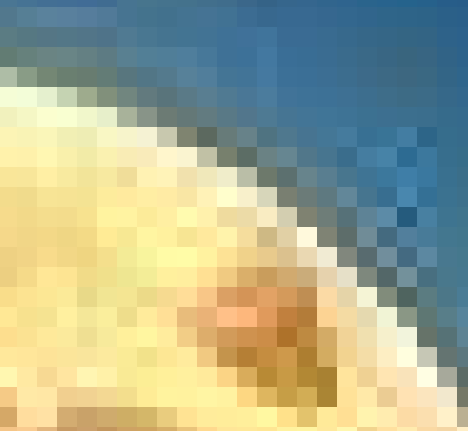
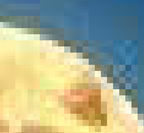
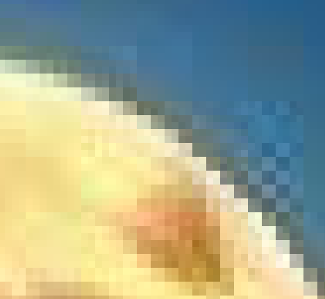
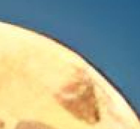
The following image serves as base. It was generated using DeepAI. When having a closer look at the image, some noise around the moon can be detected.
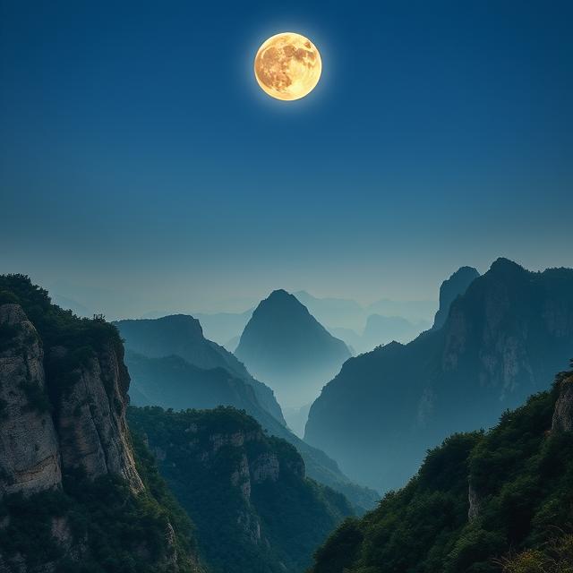
Original
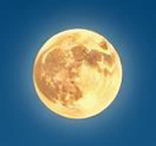
Zoomed
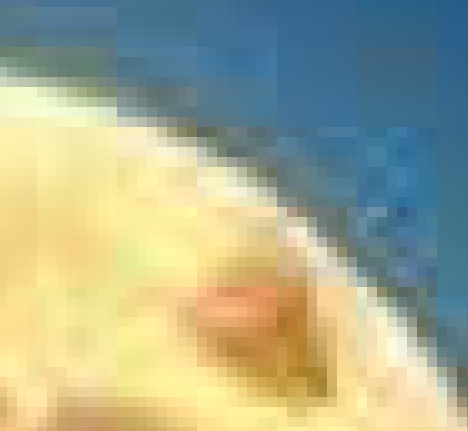
1. Nearest Neighbor Interpolation
The most basic method. Just copy the closest pixel. No blending. No subtlety. Perfect if you like your images chunky and your upscaling fast. Surprisingly, it still has its place — especially in pixel art or when you're in a rush and don't care about artifacts.
def nearest_neighbor_interpolate(img, scale):


    h, w, c = img.shape
    new_h, new_w = int(h * scale), int(w * scale)

    result = np.zeros((new_h, new_w, c), dtype=np.uint8)

    for i in range(new_h):
        for j in range(new_w):
            # Map output pixel (i,j) back to input coordinates
            x = int(np.floor(i / scale))   # Row in input
            y = int(np.floor(j / scale))   # Column in input

            # Clamp coordinates to stay in bounds
            x = min(x, h - 1)
            y = min(y, w - 1)

            # Copy nearest pixel value directly
            result[i, j] = img[x, y]

    return result
So what does this do exactly?
- For each new pixel in the enlarged image, it simply finds the closest pixel in the original image.
- No guessing, no interpolation — it just clones the nearest existing color.
- This creates that famous “blocky” look, with jagged edges and hard transitions.
Original
Upscaled (Nearest Neighbor)
To better understand what the nearest neighbor algorithm is actually doing, we created a simple 5×5 pixel test image. Each pixel has a distinct color. When upscaled, the effect of copying the nearest pixel becomes much clearer — blocks of color are stretched without blending or smoothing and the original image becomes bigger. The algorithm finds and copies the color values from the original pixel and reuses them in proportion to the scaling factor. (Side fact: On some screens the upscaled image appeared to have subtle differences in pixel colors. This can be considered hardware-related noise.)

Original 5×5 Image

Upscaled 2× (Nearest Neighbor)
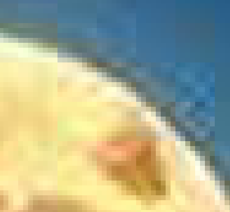
2. Box Filter Interpolation
Box filtering smooths out pixel transitions by averaging the 4 closest neighboring pixels. It’s a quick and slightly smarter method than nearest neighbor — you get fewer jagged edges, but at the cost of some sharpness.
  def box_filter_interpolate(img, scale):
    """Upscale using simple box filtering (mean of 4 nearest neighbors)."""

    h, w, c = img.shape
    new_h, new_w = int(h * scale), int(w * scale)

    result = np.zeros((new_h, new_w, c), dtype=np.uint8)

    for i in range(new_h):
        for j in range(new_w):
            # Map back to original coordinates
            x = i / scale
            y = j / scale

            # Get the 4 nearest neighbors (floor and ceil)
            x0 = int(np.floor(x))
            x1 = min(x0 + 1, h - 1)
            y0 = int(np.floor(y))
            y1 = min(y0 + 1, w - 1)

            # Average their RGB values
            pixel = (
                img[x0, y0].astype(np.uint16) +
                img[x0, y1].astype(np.uint16) +
                img[x1, y0].astype(np.uint16) +
                img[x1, y1].astype(np.uint16)
            ) // 4

            result[i, j] = pixel.astype(np.uint8)

    return result
What the algorithm does:
- For each new pixel, it calculates the average of the 4 nearest neighbors in the original image.
- This smooths transitions compared to nearest neighbor, reducing jagged edges.
- However, this method can blur fine details slightly.
Original
Upscaled (Box Filter)
Let's observe the Box Filter Effect in the 5x5 pixel version: The new color for each pixel is calculated based on the colors of the four nearest neighbors. This results in a very quirky color mix for the 5x5 test image. (Side fact: The four nearest neighbors include the original pixel itself.)
Original 5×5 Image

Upscaled 2× (Box Filter)
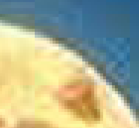
3. Bilinear Interpolation
This method uses four nearby pixels and blends them based on distance. It’s like creating a weighted average of nearby colors.
def bilinear_interpolate(img, scale):

    h, w, c = img.shape
    new_h, new_w = int(h * scale), int(w * scale)
    result = np.zeros((new_h, new_w, c), dtype=np.uint8)

    for i in range(new_h):
        for j in range(new_w):
            x = i / scale
            y = j / scale

            x0 = int(np.floor(x))
            y0 = int(np.floor(y))
            x1 = min(x0 + 1, h - 1)
            y1 = min(y0 + 1, w - 1)

            dx = x - x0
            dy = y - y0

            for k in range(c):
                a = img[x0, y0, k]
                b = img[x0, y1, k]
                c_ = img[x1, y0, k]
                d = img[x1, y1, k]

                value = (
                    a * (1 - dx) * (1 - dy) +
                    b * (1 - dx) * dy +
                    c_ * dx * (1 - dy) +
                    d * dx * dy
                )

                result[i, j, k] = int(value)

    return result
What the algorithm does:
- Each pixel in the enlarged image is calculated as a weighted average of the four closest pixels in the original image.
- The weights depend on the distance of the target pixel to each neighbor.
- This results in smooth transitions and a softer look, reducing harsh edges.
Original
Upscaled (Bilinear)
Let's examine the Bilinear Interpolation effect on a 5×5 test image. Because this method blends the four closest pixel values, each color in the result is a mix. In contrast to nearest neighbor or box filtering, bilinear blending produces a smoother appearance, even on very low-resolution images. Row-wise comparison in the test image shows large color differences due to the weighted color average of closest pixels. (Side fact: Since the algorithm only checks for the closest pixel values in the original pixel, the right neighbor, the bottom-right neighbor and the bottom neighbor, the colors don't change in the last two rows and columns.)
Original 5×5 Image

Upscaled 2× (Bilinear)
4. Bicubic Interpolation (Scipy)
Smoother than bilinear and uses a 4x4 neighborhood. It's computationally heavier but the results are cleaner — especially around edges. We will keep things short for bicubic interpolation and use Scipy's zoom().
from scipy.ndimage import zoom

def bicubic_interpolate(img, scale):
    """Upscales image using bicubic interpolation.

    This method uses 4x4 (16) nearby pixels and cubic functions to interpolate
    each new pixel value. It produces smoother results than bilinear.

    We're using SciPy's built-in `zoom()` with `order=3`:
    - order=0: Nearest
    - order=1: Bilinear
    - order=3: Bicubic
    """

    return zoom(img, (scale, scale, 1), order=3).astype(np.uint8)
What the algorithm does:
- Each new pixel is computed using a weighted average of a 4×4 neighborhood (16 pixels).
- The weights are based on cubic polynomials for smoother interpolation.
- Bicubic interpolation reduces aliasing and preserves detail better than bilinear, especially in photos with gradients or textures.
Original
Upscaled (Bicubic)
Now let’s look at the effect of bicubic interpolation on a 5×5 test image. Bicubic interpolation pulls information from a wider neighborhood (4×4), blending values using cubic functions. This produces a much smoother image compared to nearest or bilinear methods—but the result may introduce slight ringing artifacts near high-contrast edges. (Side fact: SciPy's zoom function can easily perform bilinear and nearest neighbor interpolation as well, by simply changing the order parameter.)
Original 5×5 Image

Upscaled 2× (Bicubic)
5. Lanczos Interpolation (PIL)
Lanczos interpolation is a high-quality image upscaling method that uses a windowed sinc filter to blend many surrounding pixels (usually 6–8 per axis). It creates sharp, smooth results with minimal aliasing and is often used in professional tools like Photoshop.
from PIL import Image

def lanczos_interpolate(img, scale):
    """Upscales using Lanczos resampling (high-quality).

    Lanczos uses a sinc-based kernel to interpolate pixel values,
    looking at a wide window of surrounding pixels (usually 8).

    It preserves edge sharpness better than bicubic and is often
    used in professional photo editing tools.
    """

    pil_img = Image.fromarray(img)
    new_size = (int(img.shape[1] * scale), int(img.shape[0] * scale))
    resized = pil_img.resize(new_size, resample=Image.LANCZOS)
    return np.array(resized)
What the algorithm does:
- Uses a sinc-based kernel to interpolate pixels based on many neighbors (usually 8).
- Preserves sharp edges and reduces aliasing better than other methods.
- Produces high-quality results, especially for photographs or detailed patterns.
Original
Upscaled (Lanczos)
Let's also look at the effect of Lanczos interpolation on a 5×5 pixel test image. The Lanczos filter blends across a wider area, creating very smooth transitions between color regions — sometimes even introducing small ripples (ringing artifacts) around sharp edges.
Original 5×5 Image

Upscaled 2× (Lanczos)
6. Real-ESRGAN (Deep Learning-Based)
And now, the heavyweight champ. Real-ESRGAN is a deep neural network trained on a large dataset to generate realistic high-res images from low-res ones. It doesn’t just interpolate — it hallucinates details.
It builds upon the ESRGAN framework and uses a deep convolutional architecture called RRDBNet. The model is trained on large datasets and can enhance a variety of images — from natural scenes to human faces — with remarkable detail and minimal artifacts.
Below is one way to use Real-ESRGAN in Python. Make sure to clone the repo and download the pretrained weights from the official GitHub repository.
import os
import torch
import numpy as np
from PIL import Image
from basicsr.archs.rrdbnet_arch import RRDBNet
from realesrgan import RealESRGANer

device = torch.device('cuda' if torch.cuda.is_available() else 'cpu')

# Load the original image
image_path = "img/mountain_moon_or.jpg"
img = Image.open(image_path).convert("RGB")
img_np = np.array(img)

# Define the model architecture (must match pretrained weights)
model = RRDBNet(
    num_in_ch=3, num_out_ch=3,
    num_feat=64, num_block=23,
    num_grow_ch=32, scale=4
)

model_path = "weights/RealESRGAN_x4plus.pth"  # Pretrained model

# Initialize the upscaling engine
upscaler = RealESRGANer(
    scale=4,
    model_path=model_path,
    model=model,
    tile=0,
    tile_pad=10,
    pre_pad=0,
    half=torch.cuda.is_available(),
    device=device
)

# Perform upscaling
output, _ = upscaler.enhance(img_np, outscale=4)

# Save result
Image.fromarray(output).save("img/mountain_moon_upscaled_realersgan.jpg")
We will explore how neural networks work in another blog post. For now, check out the results of Real-ESRGAN on our moon image (4× upscaled). Not only does the result look a lot more clean compared to the trials with the other algorithms - it even cleans the noise in the blue background that occures in the original image!
Original
Upscaled 4x (Real-ESRGAN)
Experiment: Real-ESRGAN on a 5×5 Pixel Image
A powerful upscaling model like Real-ESRGAN knows how to return a clean image and was even able to clear the noise in the blue background. This showcases one of the areas where simple mathematical methods struggle — neural networks can learn complex patterns from image data, essentially understanding how a clean sky should look, allowing them to perform what seems like "magic" on noisy or damaged images. But what happens if we apply Real-ESRGAN to our 5×5 test image? This could be one of those special cases where the model hasn’t been trained or doesn’t know how to interpret the unusual pattern, leading to unpredictable or unexpected results.
Original 5×5 Image

Upscaled 4× (Real-ESRGAN)
The results show how Real-ESRGAN handles unconventional input. The model smooths the image significantly, distributing colors based on the minimal structure it finds in the 5×5 input. At first glance, the result may appear slightly darker overall, but this is mostly superficial.
To test further, we apply a second and third round of 4× upscaling (totaling 16× and 64× enlargement). Since Real-ESRGAN is designed for fixed-scale enhancement, this multi-stage process demonstrates how the model continues to infer detail — even from abstract or synthetic patterns — resulting in a soft, blended image with an almost painted or dreamlike quality.

Upscaled 16× (Real-ESRGAN)
Upscaled 64× (Real-ESRGAN)
To test the consistency of Real-ESRGAN, we repeated the exact same three-stage upscaling procedure (starting from the original 5×5 test image). This was done to check whether the model introduces any randomness or variability in its output. The result: Real-ESRGAN produced identical upscaled images — both for the 4× and 64× versions — confirming that the model behaves deterministically under the same conditions.

Repeated Upscale 4× (Real-ESRGAN)

Repeated Upscale 64× (Real-ESRGAN)
In summary, Real-ESRGAN demonstrates impressive capabilities to enhance and generate high-quality details from low-resolution images, even on unusual inputs like our 5×5 test pattern. While it can produce strikingly smooth and natural results, it also behaves deterministically, consistently recreating the same output for identical inputs.
In a follow-up article, we will go deeper into how Real-ESRGAN’s neural network architecture learns and performs upscaling, why it produces consistent results on repeated runs, and we will explore additional experiments to better understand its strengths and limitations.
📌 Note: Real-ESRGAN is still widely used today and actively maintained. It performs exceptionally well for photographic content, anime, and digital art.
Wrapping Up: Why Pixel Manipulation Matters
What started as a humble for-loop scaling a few pixels can easily lead into big-league topics like:
- 🖼️ Super-resolution for restoring old photos
- 📹 AI-powered video upscaling and generation
- 🎨 Generative art and image synthesis
- 🔍 Medical imaging and scientific visualization
Whether you're building a creative tool or training the next stable diffusion model, the ability to read, modify, and create pixels is foundational. So next time you see a high-res anime face that started as a blurry blob — just remember: it all began with manipulating some numbers in an array.